Playing with Genomics Foundation Models
An overview of some early learnings from exploring how the Nucleotide Transformer from InstaDeepAI works and its downstream applications

The advent of transformer-based architectures has led to the development of foundation models across several fields, including that of genomics. However, understanding how such models can be utilised for downstream applications to solve central problems in bioinformatics can be a challenging task for those without relevant domain knowledge. I believe that whilst there is this knowledge gap between ML and biology, bridging it is precisely what unlocks our ability to solve the most important, hard problems.
On a personal note, looking into how ML is applied to genomics has been on the back-burner for some time. This self-curiosity and plausible existence of a knowledge gap have motivated me to help try to improve the context around how genomic foundation models can help in downstream applications. To do this, I’ll aim to provide a brief overview into some of these core problems within the context of a SoTA architecture, the Nucleotide Transformer. We will unpack the following:
What does genomic sequence data look like?
How does the pre-training stage of such a model work and what are some genomic specific processes that take place (e.g. k-mer tokenisation)?
What downstream problems can be solved by such models?
Code walkthrough: We will take an existing genomic foundation model and probe its ability on a central bioinformatics problem.
Some very brief context into DNA structure and transcription
You are probably aware that DNA is a fundamental molecule that encodes the instructions for how to build life. In this section, I would like to offer a brief primer on the structural components of DNA.
DNA plays a crucial role in instructing how proteins within our body are created however, it does not directly perform any cellular function. Instead, DNA is transformed into RNA which can then be passed through small, organelle machinery within our cells called ribosomes. When RNA goes through ribosomes, we then obtain functional proteins.
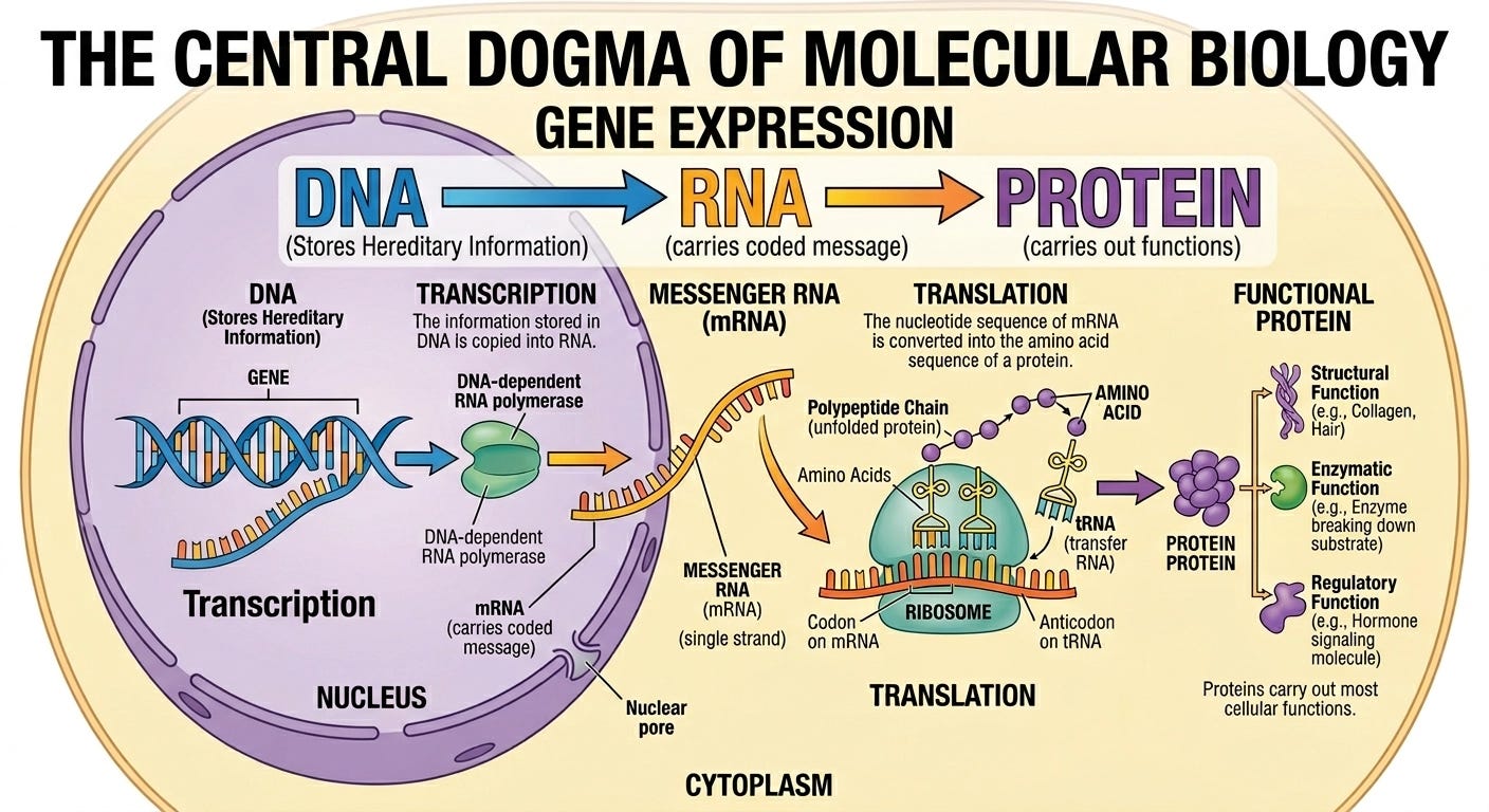
When we look at the composition of DNA molecules, they are built from small repeating units called nucleotides. Each nucleotide consists of three smaller, molecular parts: a sugar molecule, a phosphate group and importantly, a base. Within these base molecules is the encoding of actual genetic information, only formed from four different types of chemicals:
Adenine (A)
Thymine (T)
Guanine (G)
Cytosine (C).
DNA is famously double-stranded, meaning two of these nucleotide chains run alongside each other in the shape of a double helix. The strands are held together because each base on one side pairs up with a specific partner on the other, specifically:
A always bonds with T
G always bonds with C
We call these connections base pairs AND since each strand determines the other entirely, computational models typically operate over just a single-stranded representation (i.e. one strand carries all the information needed.)
From just these four bases, we can combine them in nearly endless ways to specify different proteins and in the grand scheme of matters, encode for the diverse nature of life.
An Example Problem in Machine Learning
Whilst there is a vast space of genomics related problems that can be solved through bioinformatics, I would like to use this section to help readers start to view a single, genomics problem through an ML engineering lens. To do this, we will take a look at a classification problem in genomics and then frame how a SoTA foundation model can help. My hope is that out of this section, you will gain an intuition for ML genomics sequence modelling problems and how new technology can more powerfully solve them.
Promoter Region Identification
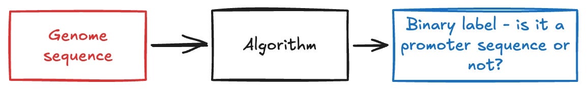
Given a genomic sequence, a core problem in ML is to determine whether the sequence is a region where transcription begins. Specifically, this is a site in a sequence where RNA polymerase can bind onto to begin creating mRNA. It is possible to frame promoter region identification as a binary classification problem that has the following structure:
Some of the earliest approaches to this problem involved identifying handcrafted, biology-informed features such as TATA sequences and CpG islands within sequences. DeePromoter is an older model that solved this problem whilst also offering a nice overview of prior approaches in their paper. I recommend reading this paper to better understand the relevance of the promoter region identification problem.
Brief Commentary on Downstream Problem and Foundation Modelling
The promoter region identification problem is just one of several other core problems in bioinformatics. For instance, genome sequences also contain splice sites which guide which regions we can copy in order to produce a functional protein. Identifying these sites is critical for understanding how pre-mRNA is processed into mature mRNA through splicing [3]. My early learnings in this topic so far have led me to believe that you can generalise how ML is applied to genomics in the following sense:
We have an input genomic sequence which put more concretely is a string of some arbitrary length
We wish to predict certain biological properties of such sequences
Looking at the downstream tasks dataset for the nucleotide transformer was quite helpful as it shows some of the other possible use cases.
Whilst it is possible to take a traditional classifier and effectively use narrow intelligence to solve each of these problems, foundation modelling is a new paradigm that can offer superior performance on such tasks. This is because foundation modelling involves a pre-training stage where we show a model vast amounts of data (even if we do not have any annotations for it and specifically train such model to recognise patterns in the data by completing some sort of pseudo-task. For example, Evo 2 is a genomic foundation model trained on 9 trillion different DNA base pairs [2]. In future, we may even be able to use these models to not just perform prediction tasks but also generate new, viable sequences of biological utility.
The core power in these genomic foundation models lies in being able to learn powerful patterns.
Then we can adapt them to further tasks such as classification problems and more recently, even designing genome sequences.
In the next section, I am going to focus on a specific example called the Nucleotide Transformer (NT) and summarise the training method for this model.
Pre-training the Nucleotide Transformer (NT)
Popular LLM models such as those of Deepseek, Claude, Gemini, etc often undergo what is called a “pre-training” stage. In this process, large amounts of data are shown to a backbone model during training which aims to learn how to extract useful features within the data through completing the task of masked language modelling. For brevity, I will not cover how transformers within an NLP context work in this article however, a good resource to learn more about this if you are interested is The Illustrated Transformer by Jay Alammar.
Foundation models in genomics can leverage the same underlying mechanics as LLMs for pre-training. The key goal of this pre-training phase is to build a network that has some understanding of the patterns present in genome sequence data it may be presented with when we adapt it for different use cases. With this in mind, we can begin to work through the construction of the Nucleotide Transformer.
Tokenisation and Vocabulary
For our transformer to work, we must first convert the input DNA sequence strings into a series of tokens that computation can be performed over. For NT, a method called k-mer tokenisation is used. Consider the following scenario:
Input Sequence: CATCGAA, K: 6
Output Tokens: <CATCGA> and <ATCGAA>
Can you see how we got these output tokens?
Our tokenisation algorithm will then break down this sequence into a series of tokens each representing continuous subsequences of 6 consecutive base pairs. Assuming this window has a stride of 1 (similar to CNNs), the tokens become <CATCGA> and <ATCGAA>. NT uses 6-mer tokenisation (i.e. k = 6) and as a result, we can also compute the resulting vocabulary length using some simple maths.
Backbone Architecture and Language Modelling Head
Using the official nucleotide_transformer_v3/model.py as a reference we can begin to understand some of the key architectural components that are used during pre-training.
Stock standard initial downsampling and feature extraction: A stem block is used for initial downsampling. Token embeddings are passed into this block here before going through a 1D convolutional tower stack.
Transformer stack: With deep features compressed by the previous 1D convolutional tower, attention blocks are stacked to learn MHSA between the input features. By default, there are 16 heads and 12 attention blocks used in this stage with a standard 512-dim embedding size.
Deconvolutional upsampling: Up until this point, we have been operating on compressed representations of the original genome sequence as this is more feasible to compute self attention across a large number of tokens in the input data. The upsampling blocks are there to help us then recover features of the original sequence length.
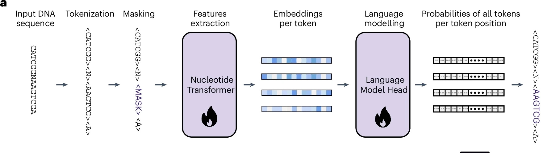
Recall that during pre-training, we are performing the task of masked language modelling in order for the transformer-based backbone to learn useful representations within the genomic data it sees. Consequently, the final module we need to connect this stack together is the language modelling (LM) head. The LM head will receive an embedding for each token and outputs logits for each token in the vocabulary, with a specific goal in mind to predict the token that has been masked upon initial input into the backbone.
This whole pipeline can be seen end-to-end in Figure 3 which is cropped from the original Nucleotide V3 paper.
Adapting to Downstream Usage
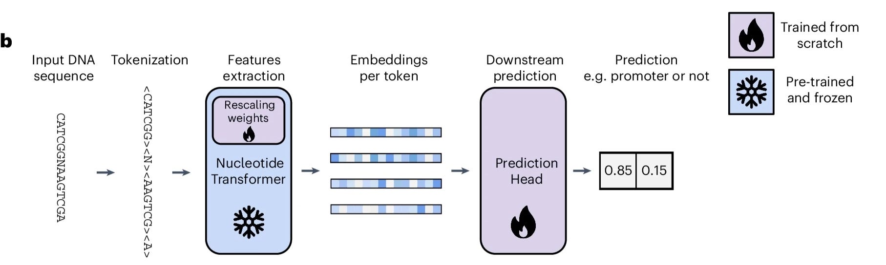
After pre-training, we can freeze the Nucleotide transformer backbone and attach a prediction head to perform domain-level tasks (Figure 4). For instance, considering the earlier example of promoter region classification, if we have an annotated dataset (smaller than pre-training data volume), we can train for this task to be performed by doing something similar to the following pseudo pytorch code:
def forward(self, tokenized_sequences: torch.Tensor):
  with torch.no_grad():
    # Disabled gradients in this context window since we use pretrained backbone
    backbone_out = self.nucleotide_transformer_backbone(tokenized_sequences)
    preds = self.mlp_prediction_head(backbone_out)
    return preds
Code Walkthrough: Using Nucleotide Transformer in Downstream Tasks
A full example of this code can be viewed here at → nt-promoter-region-classification
In this repository, my goal is to clearly demonstrate how the backbone can be applied to solve the binary classification problem of predicting if a given genome sequence (of length 300 base pairs) is a promoter region. To evaluate how well we can classify such sequences using the Nucleotide Transformer, we will use a linear probe to learn a direct mapping from the backbone outputs to a binary class.
My recommendation is to read this article section as a primer for what is contained within the codebase, followed by then working through the repo contents. I have tried to keep it lightweight and simple :)
The key files within the repository are as follows:
cli.py- Comes with a CLI script you can use to run the train.pipeline.py- Comes with a Pytorch Lightning module that can be run to train the model/model.py- This is probably the key file to view. Inside the forward pass, you will notice how the weight vector has been implemented as well as the method used to obtain attention weights which are visualised in the demo.
But first - what does the data look like?
Using the Nucleotide Transformer downstream tasks dataset, we can explore what some of the supervised data available for post-training looks like. If we consider the earlier problem of promoter region detection, let’s take a look at what the dataset for this looks like:
from datasets import load_dataset

DATASET_NAME = "InstaDeepAI/nucleotide_transformer_downstream_tasks"
TASK_NAME = "promoter_all"

ds = load_dataset(DATASET_NAME)
train_ds = ds["train"].filter(lambda x: x["task"] == TASK_NAME)
test_ds = ds["test"].filter(lambda x: x["task"] == TASK_NAME)

# Number of items in the train set
print("Number of items in the train set:")
print(len(train_ds))

# Example of item in the train set
print("Example of item in the train set:")
print(train_ds[0])
Running this block of code should output 53,276 samples in the dataset, each with a key/value structure that looks like the following:
{
  'sequence': 'ATAAA...GCACCC',
  'name': 'SLC4A1_1(-)|no_TATA|0',
  'label': 0,
  'task': 'promoter_all'
}
The main reason I wanted to spend a brief moment looking at the data is I believe directly looking at the data is one of the best ways an ML engineer can demystify how something works. In this short snippet, you can see that:
Sequences really boil down to being strings
They have certain properties, sometimes even gene names to help identify them
We can assign labels to them based on their properties (useful for supervised-settings)
Conveniently as indicated by the model card for this dataset, we can actually see this specific task only has binary labels. This means for each genomic sequence in the promoter region detection task, it is either a promoter region OR a non-promoter region. I found having a quick inspection of this data quite helpful to get my head around what modelling approaches are likely doing.
Brief Commentary on Setup and Results
In this section, I will talk about some of the key features within the codebase regarding training configurations.
Regarding model implementation: The code inside
model.pycontains a learnable weight vector which is applied to the hidden layers of the backbone outputs. Following this, a single linear layer is used to project into the binary class.Regarding compute: I trained this linear probe on my RTX 3060 at home so there were some batch size limitations in place which also caused quite a few small trains with a jumpy validation loss. As a workaround, I used a smaller learning rate than what you may typically see in other ML experiments (i.e. LR = 3e-5). Overall, reasonably happy with the
Regarding demo: After training, I used Modal for deployment and trusty Claude to help whip up the frontend. On a random side note, it is nice to see how AI coding tools can help speed up frontend work for simple demos to showcase model capabilities developed by ML engineers, researchers and hackers.
Attention Weights Visualisation
In the demo for this model, I’ve also tried to visualise the attention map for each token in the sequence. This was largely to see if there was any correlation between high attention tokens and classification result. However, this was quite tricky to determine and I suspect there were many limitations to how I was approaching it
For starters, I very quickly learnt that trying to apply the learned weight vector to each hidden layer and then pool attention across all layers OOM-ed my home GPU :(
As a workaround, I am currently just visualising the maps by pooling the attention from the most upweighted layer
Looking at the weight vector distribution is still TBD - will likely update this post if I get around to it :)
Results
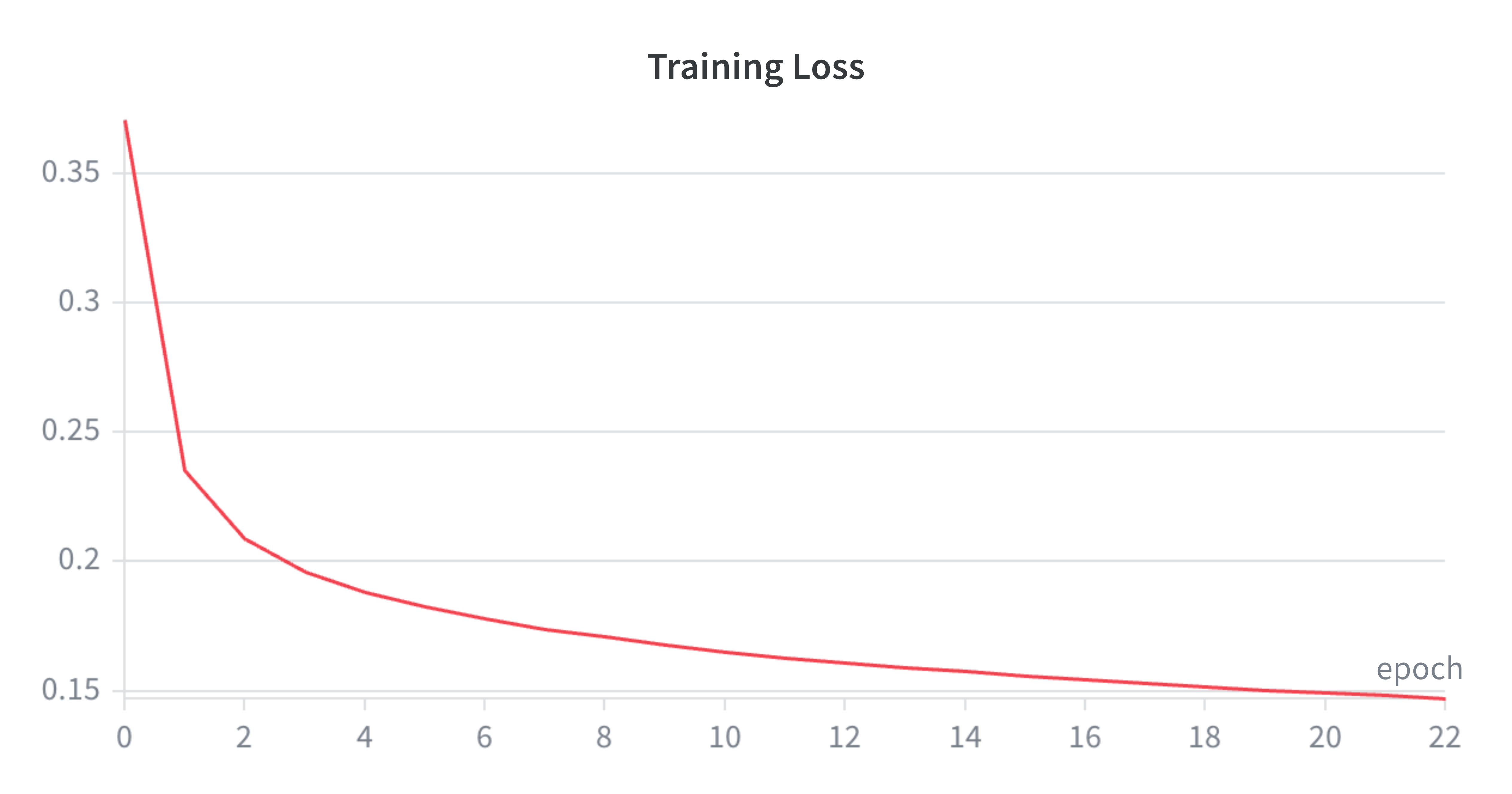
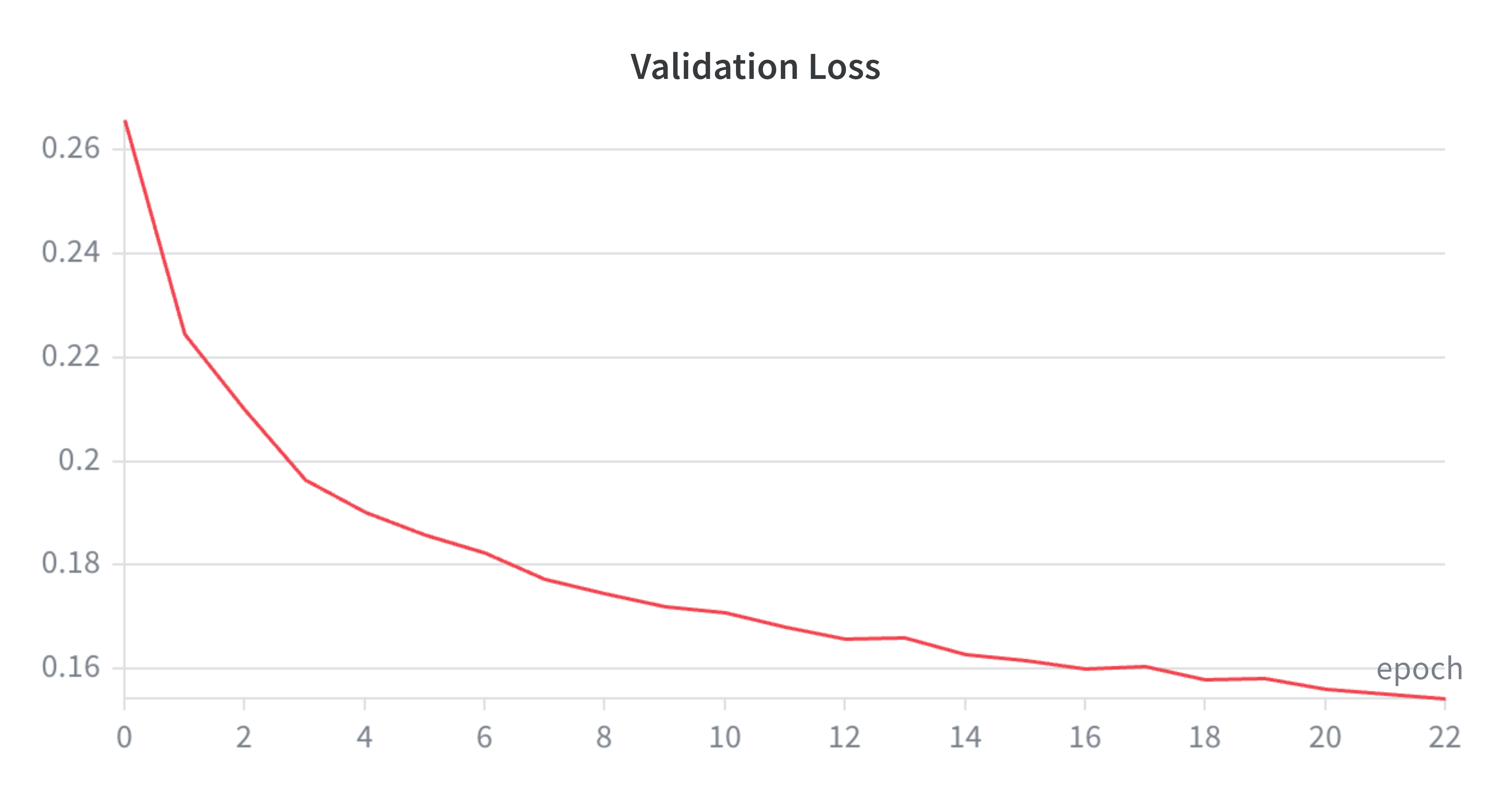
Looking at the results, its pretty cool to see how performant the backbone is!
Test AUC-ROC = 0.98474
Test Accuracy = 0.94054
Test F1-Score = 0.93973
Some pretty loss curves below as well - admittedly I was originally training this probe with early stopping (hoping it would finish by 30 epochs max). After a while, figured the plateau was happening anyway and wanted my GPU back for other shenanigans so released it and seems to be a solid training run.
Concluding Remarks
In this article, we’ve gone through quite a lot - give yourself a pat on the back if you reached this point!
My main motivation to write this article was two-fold:
Document my early learnings about how SoTA architectures in deep learning are being applied to the field of genomics, especially through considering a core biology problem.
Attempt to make this intuition more accessible by connecting an ML engineer’s lens of the world with the underlying biology domain.
Hopefully the domain feels a little more approachable now - if so, feel free to reach out, I’d love to know!
Happy genomics ML-ing folks :P
References
[1] H. Dalla-Torre et al., “Nucleotide Transformer: building and evaluating robust foundation models for human genomics,” Nature Methods, vol. 22, no. 2, pp. 287–297, Nov. 2024, doi: 10.1038/s41592-024-02523-z. Available: https://www.nature.com/articles/s41592-024-02523-z
[2] G. Brixi et al., “Genome modelling and design across all domains of life with Evo 2,” Nature, vol. 652, no. 8112, pp. 1349–1361, Mar. 2026, doi: 10.1038/s41586-026-10176-5. Available: https://www.nature.com/articles/s41586-026-10176-5
[3] R. Wang, Z. Wang, J. Wang, and S. Li, “SpliceFinder: ab initio prediction of splice sites using convolutional neural network,” BMC Bioinformatics, vol. 20, no. S23, p. 652, Dec. 2019, doi: 10.1186/s12859-019-3306-3. Available: https://pubmed.ncbi.nlm.nih.gov/31881982/